Chapter 3 Data manipulation
3.1 Collapse multiple “no” and “yes” options
Common to have to do this in GlobalSurg projects:
library(dplyr)
mydata = tibble(
  ssi.factor = c("No", "Yes, no treatment/wound opened only (CD 1)",
                 "Yes, antibiotics only (CD 2)", "Yes, return to operating theatre (CD 3)",
                 "Yes, requiring critical care admission (CD 4)",
                 "Yes, resulting in death (CD 5)",
                 "Unknown") %>%
    factor(),
  mri.factor = c("No, not available", "No, not indicated",
                 "No, indicated and facilities available, but patient not able to pay",
                 "Yes", "Unknown", "Unknown", "Unknown") %>%
    factor()
)

# Two functions make this work
fct_collapse_yn = function(.f){
  .f %>%
    forcats::fct_relabel(~ gsub("^No.*", "No", .)) %>%
    forcats::fct_relabel(~ gsub("^Yes.*", "Yes", .))
}

is.yn = function(.data){
  .f = is.factor(.data)
  .yn = .data %>%
    levels() %>%
    grepl("(No.+)|(Yes.+)", .) %>%
    any()
  all(.f, .yn)
}

# Raw variable
mydata %>%
  count(ssi.factor)
## # A tibble: 7 × 2
## ssi.factor n
## <fct> <int>
## 1 No 1
## 2 Unknown 1
## 3 Yes, antibiotics only (CD 2) 1
## 4 Yes, no treatment/wound opened only (CD 1) 1
## 5 Yes, requiring critical care admission (CD 4) 1
## 6 Yes, resulting in death (CD 5) 1
## 7 Yes, return to operating theatre (CD 3) 1# Collapse to _yn version
mydata %>%
mutate(across(where(is.yn), fct_collapse_yn, .names = "{col}_yn")) %>%
count(ssi.factor_yn)## # A tibble: 3 × 2
## ssi.factor_yn n
## <fct> <int>
## 1 No 1
## 2 Unknown 1
## 3 Yes 53.2 Filtering best practice
3.2.1 From Jamie Farrell
Particularly useful in OpenSAFELY, but should be adopted by us all.
This creates inclusion flags, and then summarises those inclusion flags in a table. This allows us to see exactly how many rows are removed at each filter step.
The inclusion flags are then used to run the final filter.
library(finalfit)
library(tidyverse)

# Utility function ----
## Ignore, just needed for the example.
fct_case_when <- function(...) {
  # uses dplyr::case_when but converts the output to a factor,
  # with factors ordered as they appear in the case_when's  ... argument
  args <- as.list(match.call())
  levels <- sapply(args[-1], function(f) f[[3]])  # extract RHS of formula
  levels <- levels[!is.na(levels)]
  factor(dplyr::case_when(...), levels=levels)
}

# Load data
colon_s = colon_s

# Create inclusion flags:
# Age over 50, male, obstruction data not missing
colon_s = colon_s %>%
  mutate(
    is_age_abover_50 = age > 50,
    is_male = sex.factor == "Male",
    obstruction_not_missing = !is.na(obstruct.factor)
  )

# Create exclusion table
flowchart = colon_s %>%
  transmute(
  c0 = TRUE,
  c1 = c0 & is_age_abover_50,
  c2 = c1 & is_male,
  c3 = c2 & obstruction_not_missing,
) %>%
  summarise(
    across(.fns=sum)
  ) %>%
  mutate(pivot_col = NA) %>%
  pivot_longer(
    cols=-pivot_col,
    names_to="criteria",
    values_to="n"
  ) %>%
  select(-pivot_col) %>%
  mutate(
    n_exclude = lag(n) - n,
    pct_all = (n/first(n)) %>% scales::percent(0.1),
    pct_exclude_step = (n_exclude/lag(n)) %>% scales::percent(0.1),
    crit = str_extract(criteria, "^c\\d+"),
    criteria = fct_case_when(
      crit == "c0" ~ "Original dataset",
      crit == "c1" ~ "  with age over 50 years",
      crit == "c2" ~ "  is male",
      crit == "c3" ~ "  obstruction data not missing",
      TRUE ~ NA_character_
    )
  ) %>%
  select(criteria, n, n_exclude, pct_all, pct_exclude_step)
flowchart
## # A tibble: 4 × 5
## criteria n n_exclude pct_all pct_exclude_step
## <fct> <int> <int> <chr> <chr>
## 1 "Original dataset" 929 NA 100.0% <NA>
## 2 " with age over 50 years" 732 197 78.8% 21.2%
## 3 " is male" 385 347 41.4% 47.4%
## 4 " obstruction data not missing" 375 10 40.4% 2.6%Now filter the dataset in one step.
3.3 Filter NA: Dropping rows where all specified variables are NA
I want to keep rows that have a value for important_a and/or important_b (so rows 1, 3, 4).
I don’t care whether whatever_c is empty or not, but I do want to keep it.
library(tidyverse)

mydata  = tibble(important_a = c("Value", NA, "Value", NA, NA),
                 important_b = c(NA, NA, "Value", "Value", NA),
                 whatever_c  = c(NA, "Value", NA, NA, NA))

mydata
## # A tibble: 5 × 3
## important_a important_b whatever_c
## <chr> <chr> <chr>
## 1 Value <NA> <NA>
## 2 <NA> <NA> Value
## 3 Value Value <NA>
## 4 <NA> Value <NA>
## 5 <NA> <NA> <NA>Functions for missing values that are very useful, but don’t do what I want are:
- This keeps complete cases based on all columns:
## # A tibble: 0 × 3
## # ℹ 3 variables: important_a <chr>, important_b <chr>, whatever_c <chr>
(Returns 0 as we don’t have rows where all 3 columns have a value).
- This keeps complete cases based on specified columns:
## # A tibble: 1 × 3
##   important_a important_b whatever_c
##   <chr>       <chr>       <chr>
## 1 Value       Value       <NA>
This only keeps the row where both a and b have a value.
- This keeps rows that have a value in any column:
## # A tibble: 4 × 3
##   important_a important_b whatever_c
##   <chr>       <chr>       <chr>
## 1 Value       <NA>        <NA>
## 2 <NA>        <NA>        Value
## 3 Value       Value       <NA>
## 4 <NA>        Value       <NA>
The third example is better achieved using the janitor package:
## # A tibble: 4 × 3
##   important_a important_b whatever_c
##   <chr>       <chr>       <chr>
## 1 Value       <NA>        <NA>
## 2 <NA>        <NA>        Value
## 3 Value       Value       <NA>
## 4 <NA>        Value       <NA>
Now, (3) is pretty close, but still, I’m not interested in row 2 - where both a and b are empty but c has a value (which is why it’s kept).
- Simple solution
A quick solution is to use ! is.na() for each variable inside a filter():
## # A tibble: 3 × 3
##   important_a important_b whatever_c
##   <chr>       <chr>       <chr>
## 1 Value       <NA>        <NA>
## 2 Value       Value       <NA>
## 3 <NA>        Value       <NA>
And this is definitely what I do when I only have a couple of these variables. But if you have tens, then the filtering logic becomes horrendously long and it’s easy to miss one out/make a mistake.
- Powerful solution:
A scalable solution is to use filter_at() with vars() with a select helper (e.g., starts with()), and then the any_vars(! is.na(.)) that was introduced in (3).
## # A tibble: 3 × 3
##   important_a important_b whatever_c
##   <chr>       <chr>       <chr>
## 1 Value       <NA>        <NA>
## 2 Value       Value       <NA>
## 3 <NA>        Value       <NA>
3.4 Vectorising rowwise procedures
We frequently have to aggregate across columns. dplyr::rowwise() is the group_by() equivalent for rows. But this is painfully slow for large datasets.
The following works beautifully and allows tidyselect of variable names.
library(tidyverse)
mydata = tibble(a = c(1,2,NA),
       b = c(2,3,NA),
       c = c(3,4,NA),
       d = c(NA,NA,NA))

mydata %>%
  mutate(s = pmap_dbl(select(., a:d), pmax, na.rm=TRUE))
## # A tibble: 3 × 5
## a b c d s
## <dbl> <dbl> <dbl> <lgl> <dbl>
## 1 1 2 3 NA 3
## 2 2 3 4 NA 4
## 3 NA NA NA NA NA3.5 Multiple imputation and IPW for missing data
Two approaches are commonly used for dealing with missing data.
Multiple imputation (MI) “fills in” missing values. Inverse probability weighting (IPW) “weights” observed values to reflect characteristics of missing data.
Missing data is discussed in detail here:https://finalfit.org/articles/missing.html
The IPW methods are taken from here: https://www.hsph.harvard.edu/miguel-hernan/causal-inference-book/
3.5.1 Data
library(finalfit)
library(tidyverse)
library(mice)

## Inspect dataset
# colon_s %>% ff_glimpse()

## Below we will use these variables to model,
## so remove missings from them and from outcome for this demonstration
explanatory = c("age",
                "sex.factor",
                "obstruct.factor",
                "perfor.factor",
                "adhere.factor",
                "nodes",
                "differ.factor",
                "rx")


## Remove existing missings
colon_s = colon_s %>%
  select(mort_5yr, explanatory) %>%
  drop_na()
Here is the truth for mortality at 5 years in these data.
##             label levels        all
##  Mortality 5 year  Alive 476 (55.7)
##                     Died 378 (44.3)
Let’s conditionally delete some outcomes.
set.seed(1234)
colon_rs = colon_s %>%
  mutate(mort_5yr = ifelse(mort_5yr == "Alive",
                           sample(c("Alive", NA_character_),
                                  size = sum(colon_s$mort_5yr == "Alive"),
                                  replace = TRUE, prob = c(0.9, 0.1)),
                           sample(c("Died", NA_character_),
                                  size = sum(colon_s$mort_5yr == "Died"),
                                  replace = TRUE, prob = c(0.85, 0.15))) %>%
           factor()
  )
The proportion that died, is now lower due to our artifically introduced reporting bias:
##     label levels        all
##  mort_5yr  Alive 423 (57.2)
##             Died 316 (42.8)
3.5.2 Multiple imputation
First, let’s use multiple imputation to “fill in” missing outcome using the existing information we have about the patient.
## Choose which variables in dataset to include in imputation.
predM = colon_rs %>%
  select(mort_5yr, explanatory) %>%
  missing_predictorMatrix(
    drop_from_imputed = c(""),
    drop_from_imputer = c(""))

# This is needed to drop from imputed
# Include for completeness, but not used here.
m0 = mice(colon_rs %>%
            select(mort_5yr, explanatory), maxit=0)
# m0$method[c("study_id")] = ""
# m0$method[c("redcap_data_access_group")] = ""

colon_rs_imputed = colon_rs %>%
  select(mort_5yr, explanatory) %>%
  mice(m = 10, maxit = 10, predictorMatrix = predM, method = m0$method,
       print = FALSE) # print false just for example

## Check output here:
# summary(colon_rs_imputed)
# plot(colon_rs_imputed )
3.5.2.1 Reduce imputed sets (mean)
As can be seen, the imputed proportion approaches that of the “true” value.
colon_rs_imputed %>%
  complete("all") %>%
  map(~ (.) %>% count(mort_5yr) %>%
        mutate(nn = sum(n),
               prop = n/nn) %>%
        select(-mort_5yr)) %>%
  reduce(`+`) / 10
## n nn prop
## 1 484.8 854 0.5676815
## 2 369.2 854 0.43231853.5.3 IPW
Rather than filling in the missing values, we can weight the observed values to reflect the characteristics of the missing data.
## Define observed vs non-observed groups
colon_rs = colon_rs %>%
  mutate(
    group_fu = if_else(is.na(mort_5yr), 0, 1)
  )

colon_rs %>%
  count(group_fu)
## group_fu n
## 1 0 115
## 2 1 739This method uses “stabilised weights”, meaning weights should have a mean of 1.
# Numerator model
fit_num = colon_rs %>%
  glmmulti("group_fu", 1)

# Denominator model
fit_dem = colon_rs %>%
  glmmulti("group_fu", explanatory)

# Check denominator model
fit_dem %>%
  fit2df()
## Waiting for profiling to be done...## explanatory OR
## 1 age 1.00 (0.99-1.02, p=0.766)
## 2 sex.factorMale 0.93 (0.62-1.38, p=0.710)
## 3 obstruct.factorYes 1.07 (0.65-1.83, p=0.803)
## 4 perfor.factorYes 4.71 (0.97-85.05, p=0.133)
## 5 adhere.factorYes 0.72 (0.43-1.26, p=0.235)
## 6 nodes 0.96 (0.91-1.01, p=0.083)
## 7 differ.factorModerate 1.61 (0.85-2.91, p=0.128)
## 8 differ.factorPoor 1.49 (0.69-3.15, p=0.301)
## 9 rxLev 1.01 (0.63-1.63, p=0.961)
## 10 rxLev+5FU 1.11 (0.68-1.82, p=0.687)colon_rs = colon_rs %>%
mutate(
p = predict(fit_num, type = "response"),
pi = predict(fit_dem, type = "response"),
weights = case_when(
group_fu == 1 ~ p / pi,
group_fu == 0 ~ (1-p) / (1-pi)
)
)
mean(colon_rs$weights)## [1] 0.9987887A weighted proportion can then be generated, which gives a very similar result to the multiple imputation.
colon_rs %>%
  mutate(
    mort_5yr_wgt = (as.numeric(mort_5yr) - 1) * weights
  ) %>%
  summary_factorlist(explanatory = c(" mort_5yr", " mort_5yr_wgt"), digits = c(4, 4, 3, 1, 1) )
## label levels all
## mort_5yr Alive 423.0 (57.2)
## Died 316.0 (42.8)
## mort_5yr_wgt Mean (SD) 0.4317 (0.5008)3.6 Store tibble metadata (factor levels and column labels) alongside a .csv file
write.rds() or save() are convenient as they save an R object including attributes such as factor levels and column labels, while write_csv() loses this information. The latter is, however, future proof, while .rda and .rds files can stop working between major R version updates.
library(tidyverse)
library(finalfit)
library(yaml)
store_data_with_metadata = function(df, filename){
write_rds(df, file = paste0(filename, ".rds"))
write_csv(df, file = paste0(filename, "_data.csv"))
# Metadata 1: Store factor levels in YAML ----
metadata = list()
# Get the names of the columns that are factors
factor_cols = select(df, where(is.factor)) %>%
colnames()
# Loop through the factor columns and store their levels
for (col_name in factor_cols) {
metadata[[col_name]] = levels(df[[col_name]])
}
write_yaml(metadata, paste0(filename, "_factor-levels.yaml"))
rm(metadata, factor_cols, col_name)
# Metadata 2: Store column labels for finalfit::ff_relabel() ----
mylabels = extract_variable_label(df) %>% unname()
mycolumns = extract_variable_label(df) %>% names()
tibble(mycolumns, mylabels) %>%
write_csv(paste0(filename, "_column-labels.csv"))
rm(mylabels, mycolumns)
}
# Example use
exampledata = tibble(record_id = 1:3,
mortality = factor(c("No", "Yes", "No")) %>% fct_expand("Died of other causes")) %>%
mutate(record_id = ff_label(record_id, "Record ID"),
mortality = ff_label(mortality, "30-day mortality"))
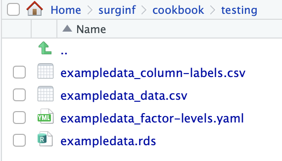
store_data_with_metadata(exampledata, "testing/exampledata")
# Usage/reapplying levels on CSV
if (FALSE){
filename = "testing/exampledata"
# Read the data from the CSV file
exampledata = read_csv(paste0(filename, "_data.csv"), guess_max = Inf)
# Read the metadata from the YAML file
exampledata_metadata = read_yaml(paste0(filename, "_factor-levels.yaml"))
# Loop through the metadata and apply the factor levels to the corresponding columns
for (col_name in names(exampledata_metadata)) {
# Check if the column exists in the reloaded tibble
if (col_name %in% names(exampledata)) {
# Convert the column to a factor with the correct levels
exampledata[[col_name]] <- factor(exampledata[[col_name]], levels = exampledata_metadata[[col_name]])
}
}
exampledata_reconst = exampledata
exampledata_csv = read_csv(paste0(filename, "_column-labels.csv"))
exampledata_labels = pull(exampledata_csv, mylabels)
names(exampledata) = pull(exampledata_csv, mycolumns)
exampledata = exampledata %>%
ff_relabel(exampledata_labels)
rm(exampledata_metadata, exampledata_reconst, exampledata_csv)
}